K-Means Image Compression in Rust
Using K-Means clustering for image compression in Rust. A visual and practical way to explore this classic machine learning algorithm.
Featured on This Week in Rust
Table of Contents
After learning about k-means clustering , I thought I understood it until I tried implementing it myself. That’s when I realized just how many details I had missed and how incomplete my theoretical understanding really was.
Implementing the core algorithm alone didn’t capture my interest. I wanted to see the algorithm’s results in action. Although I’ve spent over a decade building backend systems, there’s something satisfying about visual feedback. This led me to image compression.
While k-means clustering can be used to reduce image sizes by averaging similar colors, I’m aware there are more efficient algorithms for this purpose. However, for educational reasons, it’s an excellent way to see k-means in action.
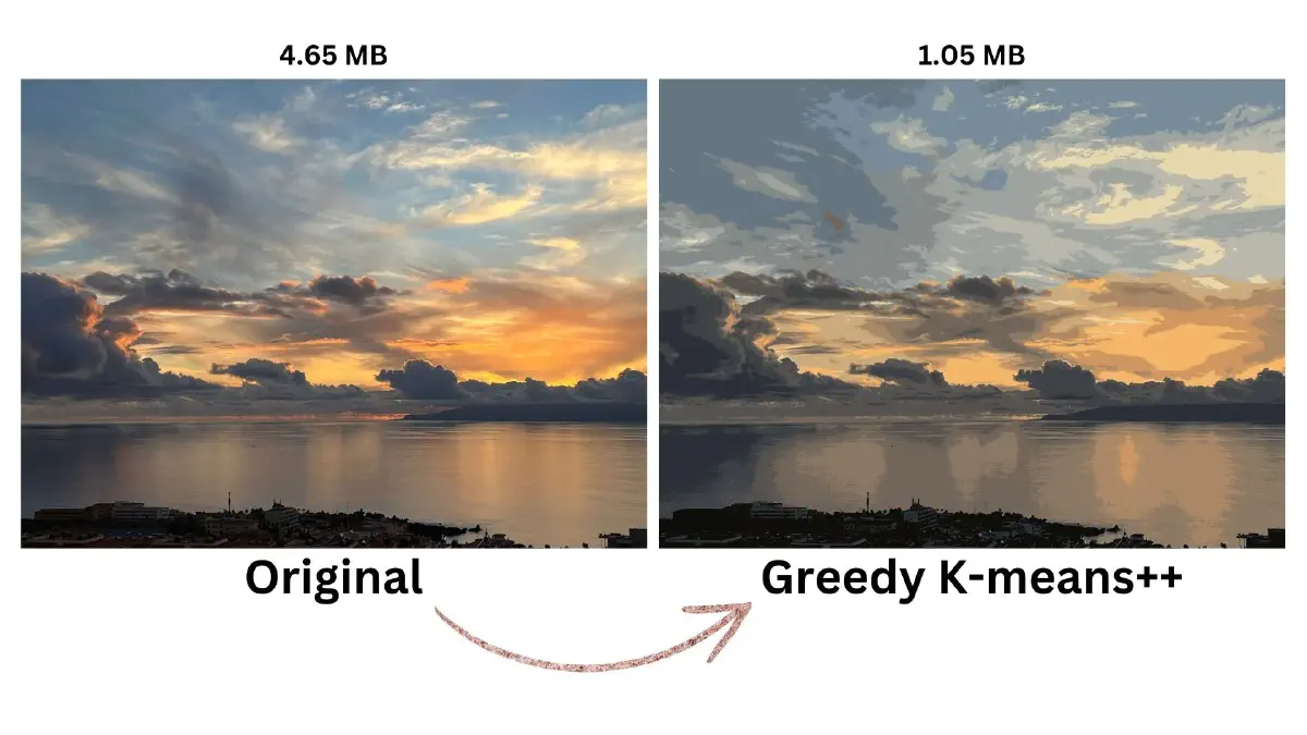
Above is a comparison of an original image (left) and its compressed version (right), which uses only 16 colors and the Greedy K-means++ initialization method for k-means.
In the sections that follow, I’ll dive deeper into other initialization methods, their implementation, and their comparative effectiveness. But first, let’s explore the fundamental components of the k-means clustering.
K-Means Clustering Algorithm
K-means clustering consists of these 5 steps:
- Initialization: Centroids are initialized using a chosen strategy. Common strategies include Forgy, MacQueen, Maximin, Bradley-Fayyad, and K-means++.
- Main Loop: The algorithm iterates until it converges or reaches the maximum number of iterations.
- Cluster Assignment: Each data point is assigned to its nearest centroid.
- Centroid Update: New centroids are calculated as the mean of the points assigned to each cluster.
- Convergence Check: The algorithm checks if the change in SSE (Sum of Squared Errors) is below a specified threshold.
function k_means_clustering(data, k, max_iterations, epsilon):
    // Initialize centroids using chosen strategy (e.g., k-means++)
    centroids = initialize_centroids(data, k)

    for iteration = 1 to max_iterations:
        // Assign each point to the nearest centroid
        clusters = assign_clusters(data, centroids)

        // Recompute centroids as the mean of assigned points
        centroids = compute_centroids(data, clusters, k)

        // Calculate the sum of squared errors (SSE)
        old_sse = sse
        sse = calculate_sse(data, clusters, centroids)

        // Check for convergence
        if (old_sse - sse) / sse < epsilon:
            break

    return centroids, clusters, sse, iteration
The pseudocode above captures the iterative process of refining cluster assignments and updating centroids to minimize the SSE, thus optimizing the grouping of data points.
Choosing Initial Centroids
Selecting initial centroids is a crucial step in the k-means algorithm because a good choice can lead to faster convergence and more effective clustering.
There has been significant research in this area, resulting in various methods for initialization . Here are some of the methods I explored for image compression, each characterized by its non-deterministic nature, meaning results may vary with each run due to their probabilistic approaches:
- Forgy: Randomly assigns each data point to one of the
kclusters, using these assignments to compute initial centroids. - MacQueen: Selects
kunique data points randomly as initial centroids. - Maximin: Iteratively selects the points that are farthest from existing centroids to ensure diversity.
- Bradley-Fayyad: Runs k-means on subsets of the data to identify effective initial centroids.
- K-means++: Chooses initial centroids with a probability proportional to their squared distance from the nearest existing centroid, enhancing cluster quality.
- Greedy K-means++: An improved version of K-means++ that evaluates multiple candidates at each step to optimize the selection.
Let’s wrap up the main k-means loop before we dive into these initialization methods in detail.
Assigning Points to Clusters
During each iteration of the k-means loop, the algorithm calculates the squared Euclidean distance between each point and every centroid. Each point is then assigned to the centroid it is closest to.
fn squared_euclidean_dist(a: &[f64], b: &[f64]) -> f64 {
    a.iter().zip(b.iter()).map(|(x, y)| (x - y).powi(2)).sum()
}

fn compute_clusters(data: &[Vec<f64>], centroids: &[Vec<f64>]) -> Vec<usize> {
    let mut result: Vec<usize> = vec![0; data.len()];
    for point in 0..data.len() {
        let mut min_dist = f64::MAX;
        for (idx, centroid) in centroids.iter().enumerate() {
            let dist = squared_euclidean_dist(&data[point], centroid);
            if dist < min_dist {
                min_dist = dist;
                result[point] = idx;
            }
        }
    }
    result
}
Updating Centroids
After assigning points to clusters, the centroids are recalculated. This is achieved by computing the average of all points within each cluster.
fn compute_centroids(data: &[Vec<f64>], clusters: &[usize], k: usize)
    -> Vec<Vec<f64>> {
    let mut result = Vec::new();
    let feature_len = data.first().unwrap_or(&vec![]).len();
    for cluster in 0..k {
        let mut centroid = vec![0f64; feature_len];
        let mut cnt = 0;
        for point in 0..data.len() {
            if clusters[point] == cluster {
                for (idx, feature) in centroid.iter_mut().enumerate() {
                    *feature += data[point][idx];
                }
                cnt += 1;
            }
        }
        if cnt > 0 {
            for feature in centroid.iter_mut() {
                *feature /= cnt as f64;
            }
        }
        result.push(centroid);
    }
    result
}
Measuring Progress with SSE
The algorithm measures its progress using the Sum of Squared Errors (SSE), which it aims to minimize. This sum is the total of the minimum squared distances between points and their respective centroids.
fn compute_sse(data: &[Vec<f64>], clusters: &[usize], centroids: &[Vec<f64>])
-> f64 {
clusters
.iter()
.zip(data.iter())
.map(|(cluster, point)|
squared_euclidean_dist(point, ¢roids[*cluster]))
.sum()
}Convergence is reached when changes in SSE are zero or so small that further iterations do not significantly improve the clusters. This condition indicates that the centroids have stabilized, and the clusters are optimally formed.
Setting a maximum number of iterations prevents the algorithm from running too long, especially when changes in SSE are negligible to make a significant difference.
Putting It All Together
Here is how the main k-means loop is implemented in Rust:
fn run_k_means(
data: &[Vec<f64>],
initial_centroids: &[Vec<f64>],
max_iters: usize,
eps: f64,
) -> (Vec<Vec<f64>>, Vec<usize>, f64, usize) {
let k = initial_centroids.len();
let mut centroids = initial_centroids.to_vec();
let mut clusters = vec![0; data.len()];
let mut sse = f64::MAX;
let mut iters = 0;
for _i in 0..max_iters {
clusters = compute_clusters(data, ¢roids);
centroids = compute_centroids(data, &clusters, k);
let prev_sse = sse;
sse = compute_sse(data, &clusters, ¢roids);
iters += 1;
if (prev_sse - sse) / sse < eps {
break;
}
}
(centroids, clusters, sse, iters)
}Now, let’s revisit the various initialization methods mentioned earlier.
K-Means Initialization Methods
There’s a lot of confusion around k-means initialization methods in the literature and practice. For instance, some sources refer to K-means++ when they’re actually implementing the Maximin method. Others incorrectly describe MacQueen’s method, which uses random initial centers, as Forgy’s.
Let’s clear up these misconceptions and explore how each method functions and how to implement them.
Forgy: Random Assignment
The Forgy method randomly assigns each data point to one of k clusters. It then calculates the centroids of these initial clusters.
pub fn init_centroids(data: &[Vec<f64>], k: usize) -> Vec<Vec<f64>> {
    let range = Uniform::from(0..k);
    let mut rng = rand::thread_rng();

    let clusters: Vec<usize> = data.iter()
        .map(|_| range.sample(&mut rng)).collect();

    compute_centroids(data, &clusters, k)
}
MacQueen: Random Sampling
The MacQueen method, also known as “Random Sampling”, selects k random data points from the dataset to serve as initial centroids.
pub fn init_centroids(data: &[Vec<f64>], k: usize) -> Vec<Vec<f64>> {
    let mut rng = rand::thread_rng();
    data.choose_multiple(&mut rng, k).cloned().collect()
}
While this method is quick and straightforward, it can sometimes result in less optimal initial centroids due to random chance.
Maximin: Spreading Centroids Apart
The Maximin method aims to spread out the initial centroids by iteratively selecting points that are farthest from the already chosen centroids. This approach tends to provide a good spread of initial centroids across the dataset.
Algorithm Steps:
- Randomly select the first centroid from the dataset.
- For each subsequent centroid:
- For each data point not yet chosen as a centroid, find its distance to the nearest existing centroid.
- Choose the data point with the maximum distance as the next centroid.
- Repeat step 2 until all
kcentroids are selected.
pub fn init_centroids(
data: &[Vec<f64>], k: usize
) -> Vec<Vec<f64>> {
let mut centroids = HashSet::new();
let mut rng = rand::thread_rng();
// Choose the first centroid randomly
centroids.insert(rng.gen_range(0..data.len()));
// Choose remaining k-1 centroids
while centroids.len() < k {
let mut max_dist = f64::MIN;
let mut centroid = 0usize;
// Find the point with maximum distance from existing centroids
for p in 0..data.len() {
if !centroids.contains(&p) {
let mut min_dist = f64::MAX;
let mut min_dist_point = p;
// Find the nearest centroid to this point
for c in ¢roids {
let dist = squared_euclidean_dist(&data[p], &data[*c]);
if dist < min_dist {
min_dist = dist;
min_dist_point = p;
}
}
// Update the max distance if this point is farther
if min_dist > max_dist {
max_dist = min_dist;
centroid = min_dist_point;
}
}
}
// Add the point with max distance as the next centroid
centroids.insert(centroid);
}
// Convert centroid indices to actual data points
centroids.iter().map(|c| data[*c].clone()).collect()
}While this method generally provides a good spread of initial centroids, it can be sensitive to outliers in the dataset. In datasets with significant outliers, this method might choose some of those outliers as initial centroids, potentially skewing the clustering results.
Bradley-Fayyad: Refined Start
The Bradley-Fayyad method, also known as the “Refined Start” algorithm, aims to find a good initial set of centroids by running k-means on multiple subsets of the data and then finding the best set of centroids among these results.
Algorithm Steps:
- Randomly partition the data into
jsubsets. - Run k-means (using MacQueen’s method for initialization) on each subset to get
jsets ofkcentroids. - Combine all these centroids into a superset.
- Run k-means
jtimes on this superset, each time initialized with a different set of centroids from step 2. - Return the set of centroids that resulted in the lowest Sum of Squared Errors (SSE).
pub fn init_centroids(
data: &[Vec<f64>],
k: usize,
j: usize,
max_iters: usize,
eps: f64,
) -> Vec<Vec<f64>> {
// Randomly partition data into j subsets
let mut rng = rand::thread_rng();
let mut points: Vec<usize> = (0..data.len()).collect();
points.shuffle(&mut rng);
let mut partitions = vec![Vec::new(); j];
let partition_size = (data.len() + j - 1) / j;
let mut partition_index = 0usize;
for p in points {
let feature = data[p].clone();
partitions[partition_index].push(feature);
if partitions[partition_index].len() == partition_size {
partition_index += 1;
}
}
// Cluster each j subset using k-means with MacQueen,
// giving j sets of intermediate centers each with k points
let mut centroids_per_partition = vec![];
let mut all_centroids = vec![];
for partition in partitions {
let initial_centroids = macqueen::init_centroids(&partition, k);
let (centroids, _, _, _) =
run_k_means(&partition, &initial_centroids, max_iters, eps);
// Combine all j center sets into a single superset
for centroid in ¢roids {
all_centroids.push(centroid.clone());
}
centroids_per_partition.push(centroids);
}
// Cluster this superset using k-means j times,
// each time initialized with a different center set j.
// Return the initialization subset j that gives the least SSE
let mut result = vec![];
let mut min_sse = f64::MAX;
for initial_centroids in centroids_per_partition {
let (_, _, sse, _) =
run_k_means(&all_centroids, &initial_centroids, max_iters, eps);
if sse < min_sse {
min_sse = sse;
result = initial_centroids;
}
}
result
}K-Means++ and Greedy K-Means++: Smarter Seeding
This method implements the k-means++ algorithm for initializing centroids, which aims to choose centroids that are both spread out and representative of the data distribution. It also includes a greedy approach to potentially improve the quality of the chosen centroids.
Algorithm Steps:
- Start by choosing the first centroid at random from the dataset.
- For each subsequent centroid:
- Calculate the distance from each point to its nearest existing centroid.
- Choose
samples_per_itercandidate points, with probability proportional to their squared distance. - For each candidate, compute the Sum of Squared Distances if it were chosen as the next centroid.
- Select the candidate that minimizes this sum.
- Repeat step 2 until
kcentroids are chosen.
pub fn init_centroids(
    data: &[Vec<f64>],
    k: usize, samples_per_iter: usize
) -> Vec<Vec<f64>> {
    // Determine the number of local centers to consider in each iteration
    let local_centers_n = if samples_per_iter > 0 {
        samples_per_iter
    } else {
        (2.0 + (k as f64).log2()).floor() as usize
    };

    let mut rng = rand::thread_rng();

    // Choose the first centroid randomly
    let initial_centroid = rng.gen_range(0..data.len());
    let mut result = vec![data[initial_centroid].clone()];

    // Initialize distances and sum of squared errors
    let mut min_dists = vec![f64::MAX; data.len()];
    let mut sse = 0f64;

    // Calculate initial distances
    for p in 0..data.len() {
        min_dists[p] = squared_euclidean_dist(&data[p], &data[initial_centroid]);
        sse += min_dists[p];
    }

    let range = Uniform::new(0.0, 1.0);

    // Choose remaining k-1 centroids
    for _ in 1..k {
        // Calculate cumulative sum of distances
        let dists_cumsum: Vec<f64> = min_dists
            .iter()
            .scan(0.0, |acc, &dist| {
                *acc += dist;
                Some(*acc)
            })
            .collect();

        // Choose candidate centroids
        let centroid_candidates: Vec<usize> = (0..local_centers_n)
            .map(|_| {
                let rand_val = rng.sample(range) * sse;
                dists_cumsum
                    .iter()
                    .position(|&dist| dist > rand_val)
                    .unwrap_or(0)
            })
            .collect();

        // Calculate distances to candidate centroids
        let mut dist_to_candidates = Vec::new();
        for candidate_index in 0..centroid_candidates.len() {
            dist_to_candidates.push(Vec::new());
            let c = centroid_candidates[candidate_index];
            for p in 0..data.len() {
                let dist = squared_euclidean_dist(&data[p], &data[c]);
                dist_to_candidates[candidate_index].push(dist);
            }
        }

        // Find the best candidate centroid
        let mut best_centroid_candidate: usize = 0;
        let mut best_sse = f64::MAX;
        let mut best_min_dists = vec![];

        for candidate_index in 0..centroid_candidates.len() {
            let mut new_min_dists = vec![];
            let mut new_sse = 0.0;
            for (dist_index, min_dist) in min_dists.iter().enumerate() {
                let dist = f64::min(*min_dist,
                                    dist_to_candidates[candidate_index][dist_index]);
                new_min_dists.push(dist);
                new_sse += dist;
            }
            if new_sse < best_sse {
                best_sse = new_sse;
                best_min_dists = new_min_dists;
                best_centroid_candidate = centroid_candidates[candidate_index];
            }
        }

        // Add the best candidate to the result
        result.push(data[best_centroid_candidate].clone());
        sse = best_sse;
        min_dists = best_min_dists;
    }

    result
}
A potential issue with k-means++ is the small but real possibility of selecting two centroids that are very close to each other due to its probabilistic nature.
The solution, often referred to as Greedy K-means++, involves selecting log(k) candidates each round for centroid selection, then choosing the candidate that minimizes the SSE. This helps to prevent the unlikely but problematic scenario of closely located centers.
I used a single function for both methods by using the samples_per_iter parameter to control the number of candidate points per iteration. For K-means++, it’s set to 1. For Greedy K-means++, it’s set to 0, and the number of candidates is determined by the formula floor(2 + log2(k)).
K-Means for Image Compression
The k-means image compression algorithm consists of 5 steps.
Step 1: Transforming Image into RGB Data
The input image is transformed into a list of RGB values, where each pixel is represented as a point in 3D space.
fn transform(image: &DynamicImage) -> Vec<Vec<f64>> {
    image
        .pixels()
        .map(|pixel| pixel.2 .0)
        .map(|rgba| {
            let mut rgb = Vec::new();
            for val in rgba.iter().take(3) {
                rgb.push(normalize(*val));
            }
            rgb
        })
        .collect()
}
Step 2: Normalizing Pixel Values
Normalizing pixel values (typically to a range of [0..1]) ensures all color channels are on the same scale. This prevents any channel from dominating the clustering process due to larger numerical values.
fn normalize(val: u8) -> f64 {
    val as f64 / 255.0
}
Additionally, many machine learning algorithms, including k-means, perform better with normalized data as it can lead to faster convergence.
Step 3: Running K-Means Clustering
The k-means algorithm described in the previous section is applied as follows:
- Each pixel is assigned to the nearest centroid.
- Centroids are recalculated based on the mean of all pixels assigned to them.
- This process repeats until convergence or a maximum number of iterations is reached.
let (centroids, clusters, sse, iters) =
    k_means::cluster(&img_data, k, &strategy);
Step 4: Denormalizing Colors
After clustering, we need to convert the compressed color values back to the original [0..255] range for standard image formats.
fn denormalize(val: f64) -> u8 {
    (val * 255.0) as u8
}
Step 5: Rebuilding the Compressed Image
Each pixel in the image is replaced with the color of its assigned centroid. That leads to the compressed image using only k colors.
fn compress(
image: &DynamicImage,
centroids: &[Vec<f64>],
clusters: &[usize],
) -> image::ImageBuffer<Rgb<u8>, Vec<u8>> {
let mut result = image::ImageBuffer::new(image.width(), image.height());
for (j, i, pixel) in result.enumerate_pixels_mut() {
let point: usize = (i * image.width() + j) as usize;
let centroid = ¢roids[clusters[point]];
let r = denormalize(centroid[0]);
let g = denormalize(centroid[1]);
let b = denormalize(centroid[2]);
*pixel = Rgb([r, g, b]);
}
result
}The image compression algorithm reduces the image’s color palette while trying to maintain overall visual similarity to the original image. Let’s apply it to a few photos and check the results.
Running the Program and Observing Compressed Images
I created a binary crate that allows you to run the image compression with the following command:
cargo run --package k_means --release -- IMAGE K STRATEGYWhere:
IMAGEis the path to your input image file.Kis the number of colors to use in the compressed image.STRATEGYis a single letter code for the centroid initialization strategy:fForgymMacQueenxMaximinbBradley-FayyadkK-means++gGreedy K-means++
Example:
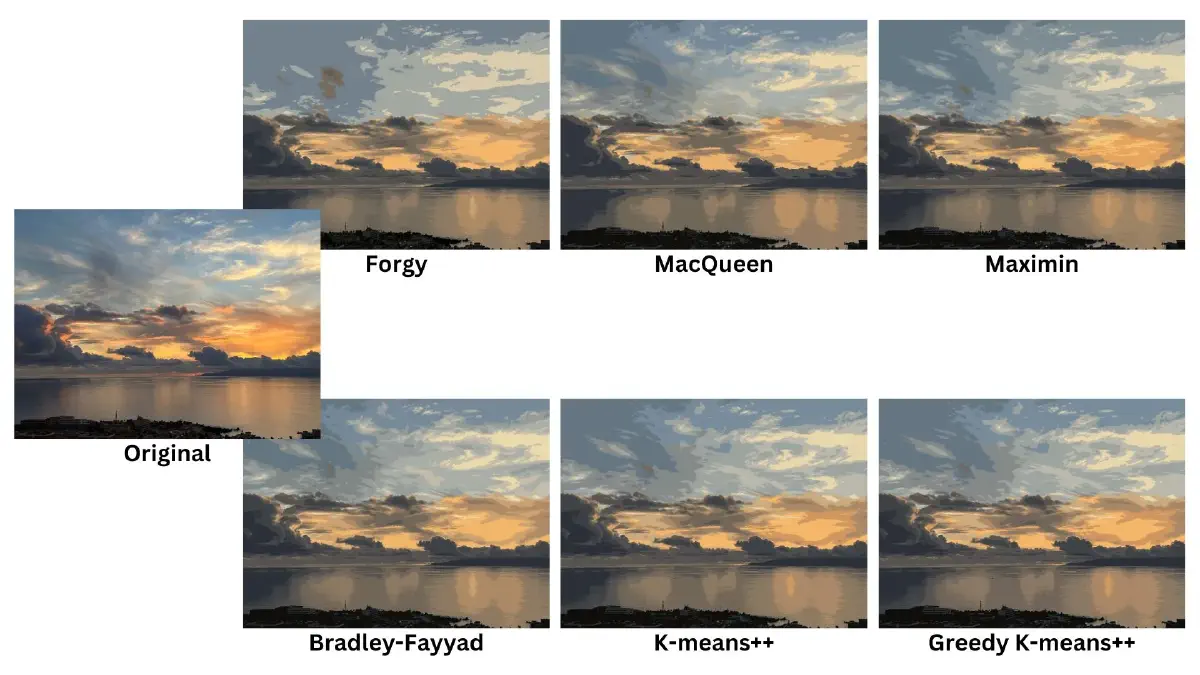
cargo run --package k_means --release -- /path/to/photo.png 16 gI compressed three different images using each initialization method with k=16. Below are results and observations.
Compression Results for a Color-Rich Photo
The compression reduced the image size from 4.65 MB to 1.05 MB, a 77.42% reduction.
| Initialization Method | Execution Time (s) | Iterations | SSE |
|---|---|---|---|
| Forgy | 63.91 | 100 | 59,622 |
| MacQueen | 41.52 | 65 | 42,087 |
| Maximin | 69.70 | 100 | 39,074 |
| Bradley-Fayyad | 97.47 | 8 | 37,709 |
| K-means++ | 51.57 | 77 | 38,160 |
| Greedy K-means++ | 34.47 | 41 | 38,164 |
The table shows a trade-off between speed and clustering quality, as measured by SSE, with different methods optimizing for one or the other. Bradley-Fayyad offers the highest quality but is the slowest compared to the other methods.
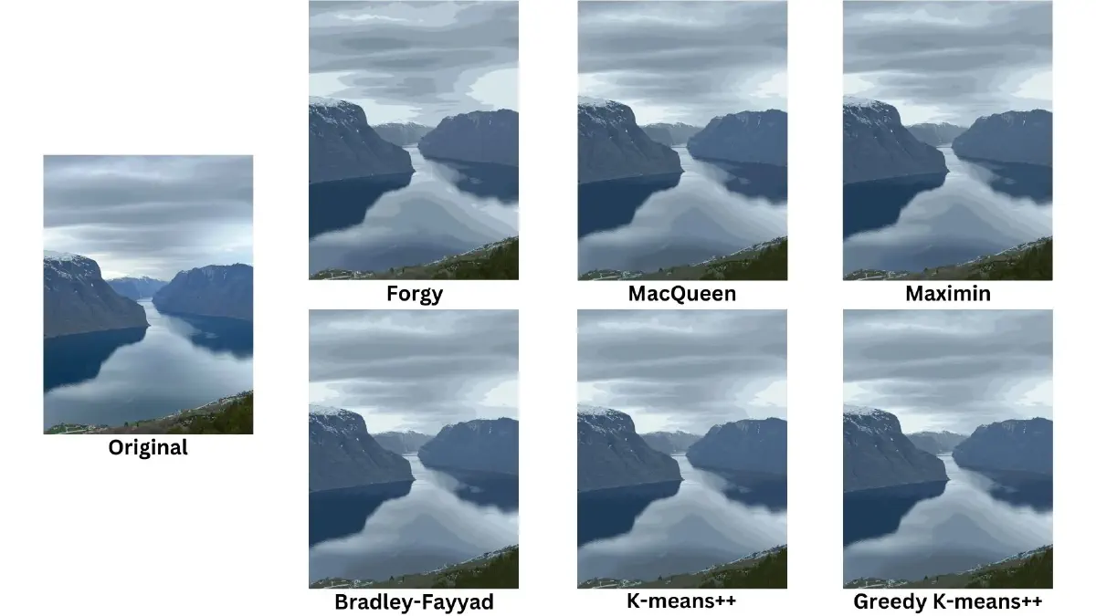
Compression Results for a Dominantly Colored Photo
The compression reduced the image size from 1.84 MB to 1.12 MB, a 39.13% reduction.
| Initialization Method | Execution Time (s) | Iterations | SSE |
|---|---|---|---|
| Forgy | 66.87 | 100 | 25,311 |
| MacQueen | 37.33 | 53 | 18,861 |
| Maximin | 44.94 | 56 | 19,132 |
| Bradley-Fayyad | 67.93 | 4 | 18,392 |
| K-means++ | 16.81 | 21 | 18,336 |
| Greedy K-means++ | 26.60 | 26 | 18,369 |
Again, there is a trade-off between execution time and clustering quality for each method. Notably, K-means++ excelled in both speed and SSE, particularly standing out in this scenario.
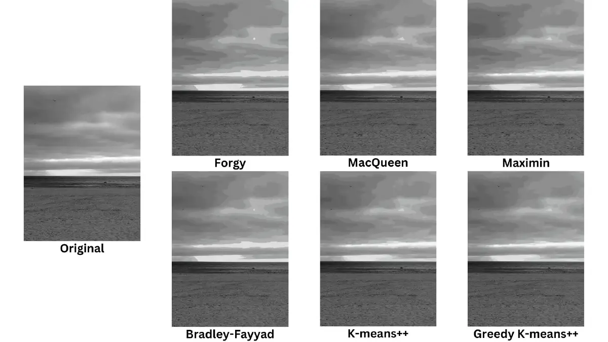
Compression Results for a Black & White Photo
The compression reduced the image size from 3.03 MB to 1.41 MB, a 53.47% reduction.
| Initialization Method | Execution Time (s) | Iterations | SSE |
|---|---|---|---|
| Forgy | 67.99 | 100 | 16,023 |
| MacQueen | 11.65 | 15 | 9,337 |
| Maximin | 25.29 | 27 | 9,488 |
| Bradley-Fayyad | 35.03 | 2 | 11,950 |
| K-means++ | 9.97 | 11 | 8,825 |
| Greedy K-means++ | 14.87 | 9 | 8,182 |
There are some interesting variations compared to the previous results. Greedy K-means++ performed well in terms of SSE, while K-means++ maintained its efficiency. The relative performance of MacQueen improved significantly in this case, showing how the effectiveness of different methods can vary depending on the specific image and randomness.
Across all tests, the Forgy method consistently underperformed, while K-means++ and Greedy K-means++ demonstrated robust performance.
Summary
When you try implementing k-means clustering yourself, you really get to understand it better and fill in any gaps in your knowledge.
Don’t just believe everything you read online, even on Wikipedia. Always check the original research papers and adjust your understanding accordingly.
K-means clustering is versatile and can be used for many other things not covered here. For image compression, the choice of initialization method doesn’t make a huge difference. Using MacQueen might result in lower quality, and Bradley-Fayyad might give a slight quality boost, but it might not be worth the extra time.
The initialization methods I used here are non-deterministic, but there are deterministic ones like PCA-Part and Var-Part. These methods require a good grasp of linear algebra, so I’ll cover them in another post once I’ve brushed up on those concepts.
Working with Rust, which isn’t my primary programming language, added to the fun. I’m open to improvements and suggestions, so feel free to contribute to the project on GitHub .